
|
|
WIDGET: A fictitious good commonly used by economic instructors to demonstrate economic principles or undertake hypothetical analyses. For example, the analysis of short-run production for a firm might be demonstrated through the production of widgets. Alternatively, the law of demand might be illustrated with a table or curve comparing the price of widgets with the quantity demanded of widgets. If such a good exists, and there is no clear evidence that widgets have every existed, it is a small mechanical device, constructed of interlocking cogs, several knobs, and at least one handle. Widgets are most often used when thingamajigs and dohickies are unavailable.
Visit the GLOSS*arama
|
|


|

|
                           PERFECT COMPETITION, LONG-RUN ADJUSTMENT: A perfectly competitive industry undertakes a two-part adjustment to equilibrium in the long run. One is the adjustment of each perfectly competitive firm to the appropriate factory size that maximizes long-run profit. The other is the entry of firms into the industry or exit of firms out of the industry, to eliminate economic profit or economic loss. The end result of this long-run adjustment is a multi-faceted equilibrium condition that price is equal to marginal cost and average cost (both short run and long run). A perfectly competitive industry adjusts to long-run equilibrium through the entry and exit of firms into and out of the industry and through each firm adjusting plant size and production to maximize economic profit in the long-run. This two-part adjustment generates equilibrium at the minimum of the long-run average cost curve, what is termed the minimum efficient scale',500,400)">minimum efficient scale.Two AdjustmentsThe two adjustments undertaken by a perfectly competitive industry in the pursuit of long-run equilibrium are:- Firm Adjustment: Each firm in the perfectly competitive industry adjustments short-run production and long-run plant size to achieve profit maximization. This adjustment entails producing the quantity that equates price (and marginal revenue',500,400)">marginal revenue) to short run marginal cost for a given plant size as well as selecting the plant size that equates price (and marginal revenue) to long-run marginal cost.
- Industry Adjustment: Firms enter and exit a perfectly competitive industry in response to economic profit and loss. If firms in the industry earn above-normal profit or receive economic profit, then other firms are induced to enter. If firms in the industry receive below-normal profit or incur economic loss, then existing firms are induced to exit. The entry and exit of firms causes the market price to change, which eliminates economic profit and loss, and leads to exactly normal profit.
The Shady Valley Zucchini IndustryConsider how this two-pronged long-run adjustment works for the hypothetical perfectly competitive Shady Valley zucchini growing industry. While zucchini growing in the real world is not really perfectly competitive, this Shady Valley industry can be used in this analysis for sake of illustration.It is assumed that the hypothetical Shady Valley zucchini industry contains a large number of relatively small firms (gadzillions of zucchini growers, each producing a handful of zucchinis each day), identical products (each zucchini is the same as every other zucchini), freedom of entry and exit (anyone can grow zucchinis with virtual no upfront cost or legal restrictions), and perfect knowledge of prices and technology (ever grower knows how to grow zucchinis and they know all relevant prices). Firm AdjustmentThis diagram displays the long-run cost curves for a representative zucchini grower named Phil. Note that because all zucchini firms have the same technology, they also have identical cost curves. So what goes for Phil goes for every other Shady Valley zucchini firm.| Firm Adjustment | 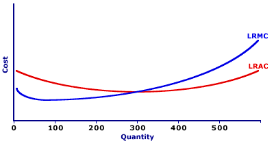
|
The LRAC is Phil's long-run average cost curve, which is an envelope of an infinite number of short-run average total cost curves. The LRMC is the long-run marginal cost curve. This indicates the change in total cost resulting from a change in production when ALL inputs, including capital and plant size, are variable.The challenge facing Phil is to identify a plant size that maximizes profit, given the going market price and marginal revenue. - Marginal Revenue: The first step is to identify the marginal revenue (that is, price) that Phil receives from selling zucchinis. This can be identified by clicking the [Marginal Revenue] button. The result is the green MR line. The MR line is horizontal and perfectly elastic at the going market price of say $4 per pound of zucchinis.
- Profit Maximization: Given this $4 market price (and marginal revenue curve), Phil's next task is to identify the quantity of zucchini production that maximizes his long-run profit. This task is accomplished by identifying the quantity in which marginal revenue is equal to marginal cost, which is the intersection of the MR and LRMC curves, and which can be found by clicking the [Profit Max] button.
- Plant Size: Once Phil determines the profit-maximizing quantity, he needs to identify the plant size (that is, size of planting bed and number of garden tools) that he can use for the short-run production of zucchinis. For each quantity of output there is one and only one plant size and corresponding set of short-run cost curves. The short-run average total and marginal cost curves for the profit-maximizing quantity selected by Phil can be revealed by clicking the [Plant Size] button.
Note that the resulting short-run average total cost curve (SRAC) just touches, or is tangent to, the long-run average cost (LRAC) at the profit-maximizing quantity. In addition, the short-run marginal cost curve (SRMC) intersects the long-run marginal cost curve (LRMC) at the same quantity.It is no coincidence the tangency between the SRAC and the LRAC corresponds with an intersection between the SRMC and LRMC. In much the same way that the long-run average cost curve is derived from a series of points from an array of short-run average total cost curves, the long-run marginal cost curve is derived from a series of corresponding points from an array of short-run marginal cost curves. The end result is that Phil is maximizing profit in the long run and he is maximizing profit in the short run. The quantity of zucchinis Phil produces is the short-run profit maximizing quantity given the plant size selected. Industry AdjustmentPhil has done all that he can do, under the circumstances. He has selected the plant size and production quantity that maximizes his profit. What more could anyone ask of a perfectly competitive firm?While Phil can adjust no further (for the time being), other firms can take action. | Industry Adjustment | 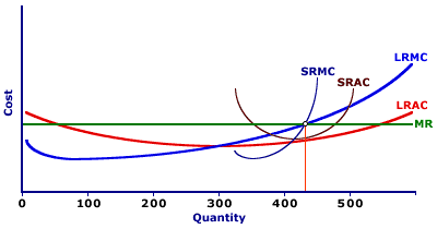
|
In particular, the plant size, profit-maximizing adjustment illustrated in this exhibit is bound to induce resource mobility. Phil's adjustment not only maximizes his profit, it generates a positive economic profit, an above-normal, a profit that exceeds that earned in other industries (such as kumquat production). Other firms, those not currently in the perfectly competitive zucchini industry, are bound to take notice. For example, a rash of kumquat growers are attracted by the above-normal profit received by Phil and other zucchini producers in the industry. They are inclined to switch from kumquats to zucchinis. What might stop the kumquat growers from growing zucchinis? Nothing. There is freedom to enter this perfectly competitive industry. The result of an increase in the number of sellers in the zucchini industry is an increase in the supply (a rightward shift of the supply curve), which results in a lower price and a lower marginal revenue received by existing firms. Click the [Enter] button to illustrate the resulting decline in marginal revenue. Note that marginal revenue (MR) shifts down until it reaches the minimum of the long-run average cost curve. At this price (and marginal revenue), all economic profit is eliminated. Price is equal to long-run average cost and the only profit generated is a normal profit. This lower price forces Phil and the other firms to re-evaluate their profit-maximizing production. What had been the long-run profit-maximizing quantity of zucchinis produced using the most efficient factory size, is no longer correct. Phil is no longer maximizing profit. Marginal revenue is not equal to marginal cost. Phil must adjust. To see how Phil adjusts his plant size, click the [Firm Readjust] button. Phil selects a new plant size that equates marginal revenue and marginal cost once again. However, this adjustment moves Phil to the minimum point of his long-run average cost curve and his minimum efficient scale of production. While this analysis has worked through the entry of firms in the industry, and the resulting decline in price, a similar story can be told for the exit of firms out of the industry in response to economic losses, and an increase in price. In both cases, every firm in the industry gravitates to the minimum efficient scale. Long-Run Equilibrium ConditionThe combination of firm and industry adjustment results in a multivariable equilibrium condition in which the price (which is also average and marginal revenue) is equal to marginal cost and average cost (both short run and long run).| P = AR = MR = MC = LRMC = ATC = LRAC |
With price (P) equal to marginal cost (MC and LRMC), each firm maximizes profit and has no reason to adjust its quantity of output or plant size. With price (P) equal to average cost (ATC and LRAC), each firm in the industry is earning only a normal profit. Economic profit is zero and there is no economic loss.
Recommended Citation:PERFECT COMPETITION, LONG-RUN ADJUSTMENT, AmosWEB Encyclonomic WEB*pedia, http://www.AmosWEB.com, AmosWEB LLC, 2000-2025. [Accessed: July 18, 2025].
Check Out These Related Terms... | | |
Or For A Little Background... | | | | | | | | | |
And For Further Study... | | | | |
Search Again?
Back to the WEB*pedia
|

|

|
ORANGE REBELOON
[What's This?]
Today, you are likely to spend a great deal of time wandering around the downtown area trying to buy either shoe laces for your snow boots or a rim for your spare tire. Be on the lookout for the happiest person in the room.
Your Complete Scope
This isn't me! What am I?
|

|
|
Woodrow Wilson's portrait adorned the $100,000 bill that was removed from circulation in 1929. Woodrow Wilson was removed from circulation in 1924.
|

|
|
"A winner is someone who recognizes his God-given talents, works his tail off to develop them into skills, and uses those skills to accomplish his goals. " -- Larry Bird, basketball player
|

|
DJ
Dow Jones
|

|
|
Tell us what you think about AmosWEB. Like what you see? Have suggestions for improvements? Let us know. Click the User Feedback link.
User Feedback
|

|