Marginal factor cost is the extra cost incurred when a firm buys one more unit of an input. It plays THE key role in the study of factor markets and the profit maximizing decision of a firm relative to marginal revenue product. A firm maximizes profit by equating marginal revenue product, the extra revenue generated from using an input, with marginal factor cost, the extra cost incurred by using the input. If these two marginals are not equal, then profit can be increased by buying more or less input.The relation between marginal factor cost and quantity of input used depends on market structure. For a perfectly competitive firm, marginal factor cost is equal to factor price and average factor cost, all of which are constant. For a monopsony, monopsonistically competitive, or oligopsony firm, marginal factor cost is greater than average factor cost and factor price, all of which increase with larger quantities of output. The constant or increasing nature of marginal factor cost is a prime indication of the market control of a firm.
Whichever market structure is involved, marginal factor cost is calculated as the change in total factor cost divided by the change in the quantity of the factor purchased, as illustrated by this equation:
| marginal factor cost | = | change in total factor cost
change in factor quantity |
If the firm is hiring the factor in a perfectly competitive factor market, then the factor price is fixed or constant and so too is marginal factor cost. If the firm is hiring the factor in an imperfectly competitive factor market, best illustrated by monopsony, then the factor price increases with larger factor quantities and so too does marginal factor cost. Perfect Competition
Perfect competition is a market structure with a large number of small participants (buyers and sellers). The good exchanged in the market is identical, regardless of who sells or who buys. Participants have perfect knowledge and perfect mobility into and out of the market. These conditions mean perfectly competitive buyers are price takers, they have no market control and must pay the going market price for all input bought.Marginal Factor Cost,
Perfect Competition |  |
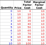
The table to the right summarizes the marginal factor cost incurred by a hypothetical buyer, Maggie's Macrame Shoppe, for hiring store clerks in a perfectly competitive labor market. Maggie's Macrame Shoppe is one of thousands of small retail stores in the greater Shady Valley metropolitan area that hires labor with identical skills. As such, Maggie pays the going wage for labor.The first column in the table is the quantity of workers hired, ranging from 0 to 10 workers. The second column is the price Maggie pays for hiring her workers, which is constant at $10 per worker. The third column is the total factor cost Maggie incurs for hiring various numbers of workers. If Maggie hires only one worker, then she pays only $10. If she hires five workers, she pays $50. In each case, total factor cost in column three is calculated as the quantity in the first column multiplied by the price in the second column.
The fourth column then presents the marginal factor cost incurred by Maggie at each level of employment. These numbers are found by dividing the change in total factor cost in the third column by the change in factor quantity in the first column. For example, when Maggie increases employment from 4 workers to 5 workers, her total factor cost increases from $40 to $50, an increase of $10. As such, the marginal factor cost of hiring the fifth worker is $10 (= $10/1). Each value in the fourth column is calculated in the same way.
The two key observations about marginal factor cost are:
- First, marginal factor cost is constant. Each level of employment results in the same $10 marginal factor cost.
- Second, marginal factor cost is equal to price (which is also average factor cost) at every level of employment. This results because Maggie is operating in a perfectly competitive labor market.
Marginal Factor Cost Curve,
Perfect Competition |  |
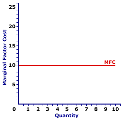
Marginal factor cost is commonly represented by a marginal factor cost curve, such as the one labeled MFC and displayed in the exhibit to the right. This particular marginal factor cost curve is that for labor hired by Maggie's Macrame Shoppe. The vertical axis measures marginal factor cost and the horizontal axis measures the quantity of input (workers). Although quantity on this particular graph stops at 10 workers, the nature of perfect competition indicates it could easily go higher.
First and foremost, the marginal factor cost curve is horizontal at the going factor price of $10. This indicates that if Maggie hires the first worker, then her total factor cost increases by $10. Alternatively, if she hires the tenth worker, then her total factor cost increases by $10. Should she hire a hundredth worker, then she might move well beyond the graph, but her total factor cost increases by $10.
The "curve" is actually a "straight line" because Maggie is a price taker in the labor market. She pays $10 for each worker whether she hires 1 worker or 10 workers or 100 workers. Her extra factor cost of hiring an extra worker is always $10. The constant price is what makes Maggie's marginal factor cost curve a straight line, and which indicates that Maggie has no market control.
Monopsony, Oligopsony, and Monopsonistic Competition
For market structures like monopsony, oligopsony, and monopsonistic competition that have some degree of market control on the buying side and are price makers rather than price takers, marginal factor cost is a little different. Market control means these market structures face positively-sloped supply curves. As such, the price received is not fixed, but depends on the quantity of the input bought.Marginal Factor Cost,
Monopsony |  |
The table to the right summarizes the marginal factor cost received by another hypothetical firm, OmniKing Island Resort. This firm is the only employer of labor on a small tropical island. As the only employer on the island, OmniKing is a monopsony with extensive market control and it faces a positively-sloped supply curve. To employ more workers, OmniKing must pay a higher price.This table is comparable to that for perfect competition. The first column in the table is the quantity of workers hired, ranging from 0 to 10 workers. The second column is the price OmniKing pays for hiring workers, which increases from a low of $5 for 0 workers to a high of $15 for 10 workers. The third column is the total factor cost OmniKing incurs for hiring various numbers of workers. If OmniKing hires only one worker, then it pays only $5. If it hires five workers, it pays $50. In each case, total factor cost in column three is calculated as the quantity in the first column multiplied by the price in the second column.
The fourth column then presents the marginal factor cost incurred by OmniKing at each level of employment. These numbers are found by dividing the change in total factor cost in the third column by the change in factor quantity in the first column. For example, the total factor cost of hiring the fifth worker over the fourth increases from $36 to $50, resulting in a marginal factor cost of $14 (=$14/1).
The two key observations about marginal factor cost are:
- First, marginal factor cost is not constant, but increases as the level of employment increases.
- Second, marginal factor cost is greater than price (which is also average factor cost) at every level of employment. Marginal factor cost is greater than price because OmniKing must increase the price paid to all workers when it raises the price to hire an additional worker.
Marginal Factor Cost Curve,
Monopsony |  |
The marginal factor cost curve for firms with market control looks a little different than that for perfect competition. The marginal factor cost curve (MFC) for OmniKing Island Resort is displayed in the exhibit to the right. Key to this curve is that OmniKing is a monopsony buyer of workers and thus faces a positively-sloped supply curve. Larger quantities of input can be had only with higher prices.The vertical axis measures marginal factor cost and the horizontal axis measures the quantity of input (workers). Although quantity on this particular graph stops at 10 workers, it could go higher.
This curve indicates that if OmniKing hires the first worker, then marginal factor cost is $6. Alternatively, if it hires the tenth worker, then marginal factor cost is $24.
For reference, the factor supply curve (and average factor cost curve, AFC) is also presented in the exhibit. The key observation is that the positively-sloped marginal factor cost curve (MFC) lies above the supply curve (AFC) facing OmniKing for hiring labor. The positioning of the marginal factor cost curve above the average factor cost curve reflects the mathematical relation between an average and a marginal.
Although this marginal factor cost curve, and preceding table of marginal factor cost numbers, is based on the employment activity of OmniKing Island Resort, a well-known monopsony firm, it works for any buyer with market control. Monopsonistic competition and oligopsony firms that also face positively-sloped supply curves generate comparable total factor costs.
MARGINAL FACTOR COST, AmosWEB Encyclonomic WEB*pedia, http://www.AmosWEB.com, AmosWEB LLC, 2000-2025. [Accessed: July 18, 2025].


