|
|
COMPETITIVE FORCES: Forces in the marketing environment that are based on competition among customers and competition with other firms. As the organization looks out at its business environment, competition is a critical factor. Who is buying goods and services and who is providing them to those customers? Are there many competitors or are there just a few? Maybe none. Knowing what competitive forces exist helps an organization develop strategic planning to attract customers.
Visit the GLOSS*arama
|
|


|

|
                           MONOPOLISTIC COMPETITION, LONG-RUN ADJUSTMENT: A monopolistically competitive industry undertakes a two-part adjustment to equilibrium in the long run. One is the adjustment of each monopolistically competitive firm to the appropriate factory size that maximizes long-run profit. The other is the entry of firms into the industry or exit of firms out of the industry, to eliminate economic profit or economic loss. The end result of this long-run adjustment is two equilibrium conditions--one for profit maximization, the other for zero economic profit. A monopolistically competitive industry adjusts to long-run equilibrium through the entry and exit of firms into and out of the industry and through each firm adjusting plant size and production to maximize economic profit in the long-run. Because a monopolistically competitive firm has market control and faces a negatively-sloped demand curve, this two-part adjustment generates equilibrium on the negatively-sloped segment of the long-run average cost curve. This equilibrium is in the economies of scale range of production that falls short of the minimum efficient scale.Two AdjustmentsThe two adjustments undertaken by a monopolistically competitive industry in the pursuit of long-run equilibrium are:- Firm Adjustment: Each firm in the monopolistically competitive industry adjusts short-run production and long-run plant size to achieve profit maximization. This adjustment entails producing the quantity that equates marginal revenue',500,400)">marginal revenue to short run marginal cost for a given plant size as well as selecting the plant size that equates marginal revenue to long-run marginal cost.
- Industry Adjustment: Firms enter and exit a perfectly competitive industry in response to economic profit and loss. If firms in the industry earn above-normal profit or receive economic profit, then other firms are induced to enter. If firms in the industry receive below-normal profit or incur economic loss, then existing firms are induced to exit. The entry and exit of firms causes the market price to change, which eliminates economic profit and loss, and leads to exactly normal profit.
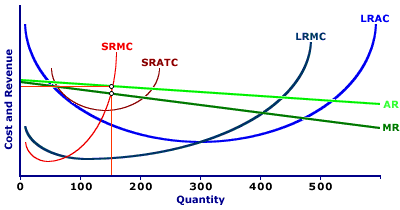
The Shady Valley Restaurant IndustryConsider how this two-pronged long-run adjustment works for the hypothetical monopolistically competitive Shady Valley restaurant industry. It is assumed that the Shady Valley restaurant industry contains a large number of relatively small firms (thousands of restaurant owners, each with a small quantity of output each day), similar but not identical products (each produces food, but the meals differ from restaurant to restaurant), relative ease of entry and exit (anyone can set up a restaurant with little no upfront cost and few legal restrictions), and extensive knowledge of prices and technology (ever restaurant knows how to prepare meals and they are aware of relevant prices). Firm AdjustmentThis diagram displays the long-run cost curves for a representative restaurant, Manny Mustard's House of Sandwich. Note that because the restaurant firms have similar technology, they also have similar cost curves. So what goes for Manny Mustard goes for every other Shady Valley restaurant.| Firm Adjustment |  |
The LRAC is Manny's long-run average cost curve, which is an envelope of an infinite number of short-run average total cost curves. The LRMC is the long-run marginal cost curve. This indicates the change in total cost resulting from a change in production when ALL inputs, including capital and plant size, are variable.- Short-Run Equilibrium: The current situation shows Manny maximizing short-run profit given a relatively small plant size. His production level is 150 meals per day. This production level, however, does not maximize long-run profit. Manny's task is to identify the long-run profit-maximizing production level.
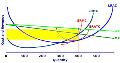
- Long-Run Profit Maximization: To maximize long-run profit, Manny needs to find the production level that equates marginal revenue and long-run marginal cost, which is the intersection of the MR and LRMC curves. This can be highlighted by clicking the [Profit Max] button. The resulting quantity is approximately 405 meals per day.
- Plant Size: Once Manny determines the profit-maximizing quantity, he needs to identify the plant size (that is, size of his restaurant, number of tables, etc.) that he can use for the short-run production of food. For each quantity of output there is one and only one plant size and corresponding set of short-run cost curves. The short-run average total and marginal cost curves for the profit-maximizing quantity selected by Manny can be revealed by clicking the [Plant Size] button.
- Economic Profit: At this production level, achieved with the larger plant size, Manny maximizes long-run profit. The extent of this profit can be highlighted in yellow with a click of the [Economic Profit] button.
Note that the resulting short-run average total cost curve (SRAC) just touches, or is tangent to, the long-run average cost (LRAC) at the profit-maximizing quantity. In addition, the short-run marginal cost curve (SRMC) intersects the long-run marginal cost curve (LRMC) at the same quantity.It is no coincidence that the tangency between the SRAC and the LRAC corresponds with an intersection between the SRMC and LRMC. In much the same way that the long-run average cost curve is derived from a series of points from an array of short-run average total cost curves, the long-run marginal cost curve is derived from a series of corresponding points from an array of short-run marginal cost curves. The end result is that Manny maximizes profit in the long run and he maximizes profit in the short run. The quantity of output Manny produces is the short-run profit maximizing quantity given the plant size selected. Industry AdjustmentManny has done all that he can do, under the circumstances. He has selected the plant size and production quantity that maximizes his profit. What more could anyone ask of a monopolistically competitive firm?While Manny can adjust no further (for the time being), other firms can take action. | Industry Adjustment |  |
In particular, the plant size, profit-maximizing adjustment illustrated in this exhibit is bound to induced resource mobility. Manny's adjustment not only maximizes his profit, it generates a positive economic profit, an above-normal profit, a profit that exceeds that earned in other industries (such as macrame sales or bookstores). Other firms, those not currently in the monopolistically competitive restaurant industry, are bound to take notice. For example, a rash of bookstores might be attracted by the above-normal profit received by Manny and other restauranteers in the industry. They are inclined to switch from book sales to food sales. And what might stop the book stores from starting restaurants? Almost nothing. There is relative freedom to enter this monopolistically competitive industry. - Entry of New Firms: The result of an increase in the number of producers in the restaurant industry is an increase in the supply (a rightward shift of the supply curve), which results in relatively less demand for each existing firm. To see what this means for Manny's production, click the [More Firms] button.
Note that average revenue (AR) and marginal revenue (MR) curves shift down until the average revenue curve just touches the long-run average cost curve (LRAC). At this average revenue (and price) all economic profit is eliminated. Price is equal to long-run average cost and the only profit generated is a normal profit.
- Plant Size Readjustment: This lower price forces Manny (and the other firms) to re-evaluate their profit-maximizing production and plant size. What had been Manny's long-run profit-maximizing production level using the larger restaurant, is no longer correct. Manny is no longer maximizing profit. Marginal revenue is not equal to marginal cost. Manny must adjust.
To see how Manny adjusts his plant size, click the [New Plant Size] button. Manny selects a new plant size that equates marginal revenue and marginal cost once again. However, this adjustment moves Manny to a smaller level of production and point of tangency on the LRAC curve.
While this analysis has worked through the entry of firms in the industry, and the resulting decline in demand, a similar story can be told for the exit of firms out of the industry in response to economic losses, and an increase in demand for the firms that remain. In both cases, every firm in the industry gravitates to the zero economic profit and a tangency between the average revenue and long-run average cost curves.Long-Run Equilibrium ConditionsThe combination of firm and industry adjustment results in a two equilibrium conditions. The profit-maximizing condition is that marginal revenue is equal to marginal cost (both short run and long run). The zero economic profit condition is that price (and average revenue) is equal to average cost (both short run and long run).| MR = MC = LRMC | | P = AR = ATC = LRAC |
With marginal revenue (MR) equal to marginal cost (MC and LRMC), each firm maximizes profit and has no reason to adjust its quantity of output or plant size. With price (P) equal to average cost (ATC and LRAC), each firm in the industry is earning only a normal profit. Economic profit is zero and there is no economic loss.Key to these conditions is that they are NOT equal. Because price is not equal to marginal revenue in monopolistic competition, average cost is not equal to marginal cost. The only production level in which average cost is equal to marginal cost (both short run and long run) is at the minimum efficient scale of production, the bottom of the long-run average cost curve. The only way to achieve this production level is the equality between price and marginal revenue. This equality is only achieved for perfect competition.

Recommended Citation:MONOPOLISTIC COMPETITION, LONG-RUN ADJUSTMENT, AmosWEB Encyclonomic WEB*pedia, http://www.AmosWEB.com, AmosWEB LLC, 2000-2025. [Accessed: July 18, 2025].
Check Out These Related Terms... | | |
Or For A Little Background... | | | | | | | | | |
And For Further Study... | | | | | | | |
Search Again?
Back to the WEB*pedia
|


|

|
PURPLE SMARPHIN
[What's This?]
Today, you are likely to spend a great deal of time flipping through mail order catalogs trying to buy either a flower arrangement for your aunt or a birthday greeting card for your uncle. Be on the lookout for rusty deck screws.
Your Complete Scope
This isn't me! What am I?
|

|
|
Woodrow Wilson's portrait adorned the $100,000 bill that was removed from circulation in 1929. Woodrow Wilson was removed from circulation in 1924.
|

|
|
"A winner is someone who recognizes his God-given talents, works his tail off to develop them into skills, and uses those skills to accomplish his goals. " -- Larry Bird, basketball player
|

|
ACT
Advance Corporation Tax
|

|
|
Tell us what you think about AmosWEB. Like what you see? Have suggestions for improvements? Let us know. Click the User Feedback link.
User Feedback
|


|


